Tracking in Mixed Reality
From Cameras to Robust Visual Tracking
Étienne Peillard – IMT Atlantique
🎯 Course Objectives
By the end of this lecture, you should be able to:
- Explain what tracking means in Mixed Reality
- Understand how cameras form digital images
- Connect image processing to feature detection
- Understand how features enable 6DoF tracking
- See the link with the practical lab (feature detection for tracking)
PART A — Why Tracking in Mixed Reality?
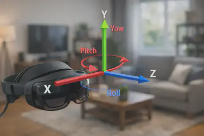
What is Tracking in Mixed Reality?
Tracking = continuous estimation of pose:
- Position (x, y, z)
- Orientation (roll, pitch, yaw)
This applies to:
- The camera/headset
- The user’s body
- Objects in the environment
- Sometimes the entire scene (SLAM)
Why is Tracking Critical in MR?
Because MR requires spatial alignment between:
- The real world (captured by sensors)
- The virtual world (rendered by the engine)
If tracking is wrong:
- Virtual objects drift
- Registration breaks
- The experience feels “fake” or unstable
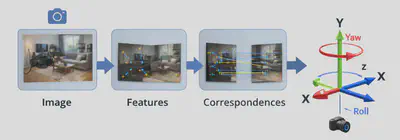
The Registration Problem
Core question:
Given an image from a moving camera, how do we estimate its 6DoF pose in the real world?
Conceptual pipeline:
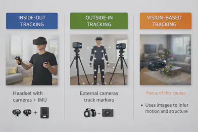
Three Families of Tracking in XR
Tracking and Latency
Good tracking must be:
- Accurate
- Low-latency
- Robust to occlusion
- Stable over time
Why? Because MR rendering depends on it in real time.
PART B — From Camera to Digital Image
Cameras as Sensors in XR
A camera is a physical sensor that:
- Captures light from the environment
- Converts it into a digital image
- Introduces limitations that affect tracking
Key issues:
- Discretization
- Aliasing
- Noise
- Limited dynamic range
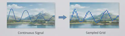
Discretization of Images
The real world is continuous.
A digital image is sampled on a grid of pixels.
This creates:
- Loss of detail
- Potential aliasing
- Dependence on resolution
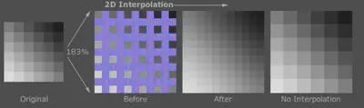
Interpolation
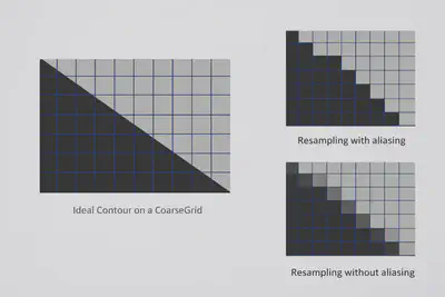
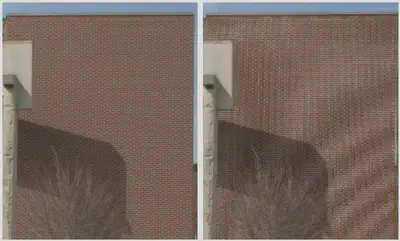
Aliasing and Moiré
If sampling is too coarse:
- High-frequency patterns create artifacts (moiré)
- Edges look jagged (aliasing)
This matters for tracking:
- Artifacts can confuse feature detectors
Aliasing
Moiré
Nyquist–Shannon Theorem
To properly sample a signal: Sampling frequency ≥ 2 × highest frequency in the signal
If violated → aliasing appears.
Color Quantization
Real light is continuous.
Digital images use a finite number of values:
- Typically 8-bit per channel (0–255)
- RGB representation
This limits precision in low-light conditions.
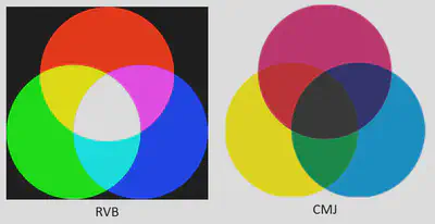
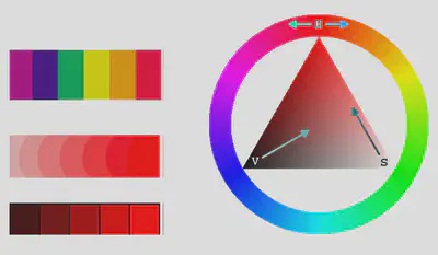
From RGB to Perception
Different color spaces exist:
- RGB (device-oriented)
- HSV (more aligned with human perception)
- Hue
- Saturation
- Value (brightness)
Useful in some tracking pipelines.
PART C — Projective Geometry (Core for Tracking)
Why Geometry Matters for Tracking
Tracking is fundamentally projective geometry.
We need to model:
- How 3D points project onto a 2D image
- How camera motion affects this projection
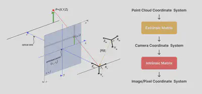
Intrinsic Parameters (K)
Describe the internal properties of the camera:
- Focal length
- Principal point
- Pixel aspect ratio
Fixed for a calibrated camera.
Extrinsic Parameters (R, t)
Describe the pose of the camera in the world:
- Rotation matrix R
- Translation vector t
👉 This is what tracking estimates.
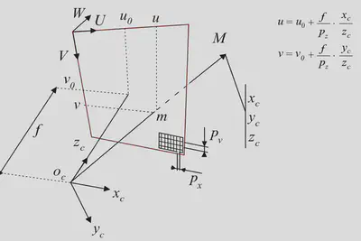
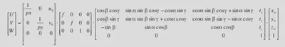
The Projection Model (Simplified)
The core equation:
u = K [R | t] X
Where:
- X = 3D point in the world
- u = 2D pixel in the image
- K = intrinsics
- [R|t] = camera pose (tracking result)
Intuition of the Projection
- Transform 3D point from world to camera space (R, t)
- Project onto image plane (K)
- Obtain pixel coordinates (u)
This is the mathematical backbone of visual tracking.
PART D — Image Processing as a Precursor to Tracking
Why Image Processing for Tracking?
Three main goals:
- Reduce noise → more stable features
- Enhance structures → clearer edges/corners
- Normalize images → robustness across lighting changes
Grayscale Conversion
Most feature detectors work on grayscale images.
Classic formula:
Y = 0.299R + 0.587G + 0.114B
Reduces complexity while preserving structure.
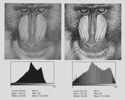
Histogram Equalization
Improves contrast:
- Makes details more visible
- Helps feature detection in low-contrast images
Useful in challenging lighting conditions.
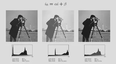
Contrast and Brightness Adjustment
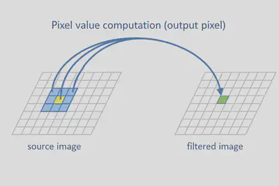
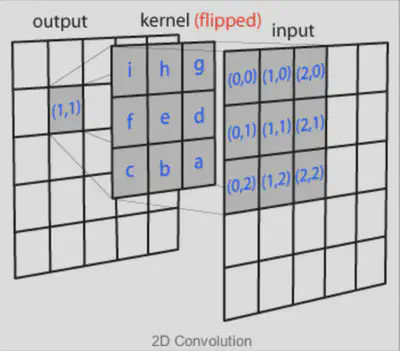
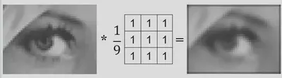
Convolution — The Key Tool
A sliding kernel is applied over the image.
Each pixel becomes a weighted sum of its neighbors.
This enables:
- Blurring
- Edge detection
- Feature enhancement
Simple Blur
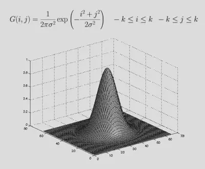
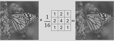
Gaussian Blur
Used to:
- Reduce high-frequency noise
- Smooth the image before detecting features
Important for robust tracking.
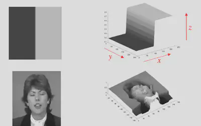
Gradients and Edges
Edges correspond to strong intensity changes.
We compute gradients using filters such as:
- Sobel
- Prewitt
Edges help locate meaningful structures.
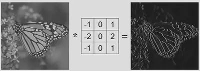
Sobel Filter
$f’(i)=\frac{f_{i+1}-f_{i-1}}{2}\ \text{is equivalent to}\ [\tfrac12,\ 0,\ -\tfrac12]$
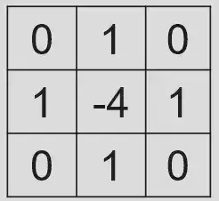
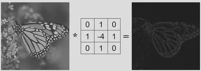
Laplacian (Second-Order Derivative)
Detects regions of rapid change:
- Useful for feature detection
- Highlights corners and fine details
The standard discrete Laplacian is written:
$\nabla^2 f(i,j)=f_{i+1,j}+f_{i-1,j}+f_{i,j+1}+f_{i,j-1}-4f_{i,j}$
This corresponds to the kernel:
From Image Processing to Features
At this stage, we have a cleaned and enhanced image.
Next step: 👉 Detect meaningful points for tracking.
PART E — Feature Detection for Visual Tracking
What is a Feature?
A feature is a distinctive image pattern that can be reliably detected and matched across frames.
Examples:
- Corners
- Blobs
- Edges

What Makes a Good Feature?
A good feature should be:
- Local (robust to occlusion)
- Invariant (to translation, rotation, scale)
- Robust (to noise, lighting changes)
- Distinctive (easy to match)
- Repeatable (found again in next frame)
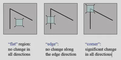
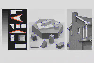
Why Corners are Ideal
Corners are:
- Stable across viewpoints
- Well-localized in both x and y
- Highly informative for motion estimation
Moravec Corner Detector (1977)
Idea:
- Measure how much intensity changes when shifting a small window in different directions.
Average intensity variation for a small displacement ((u,v))
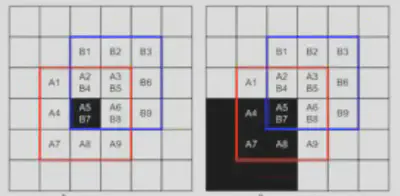
$E(u,v)=\sum_{x,y} w(x,y),(I(x+u,y+v)-I(x,y))^2$
- (w) specifies the considered neighborhood (value 1 inside the window and 0 outside);
- (I(x,y)) is the intensity at pixel ((x,y)).
Results
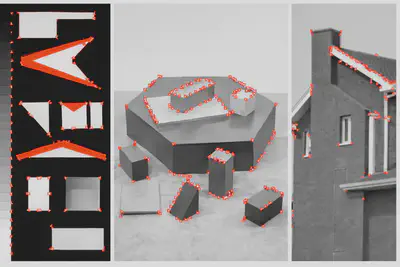
Limitation:
- Not rotation invariant.
Harris Corner Detector (1988)
Improvement over Moravec:
- Uses image gradients
- More robust
- Rotation invariant
Widely used in vision-based tracking.
Average intensity variation for a small displacement $(u,v)$
$E(x,y)=\sum_{u,v} w(u,v),|I(x+u,y+v)-I(x,y)|^2$
- $w$ specifies the considered neighborhood (value 1 inside the window, 0 outside);
- $I(x,y)$ is the intensity at pixel $(x,y)$.
Taylor expansion
$I(x+u,y+v)=I(x,y)+u\frac{\partial I}{\partial x}(x,y)+v\frac{\partial I}{\partial y}(x,y)+o(u^2,v^2)$
Neglecting $o(u^2,v^2)$:
$E(x,y)=\sum_{u,v} w(u,v)\left|u\frac{\partial I}{\partial x}(x,y)+v\frac{\partial I}{\partial y}(x,y)\right|^2$
Quadratic form
Average intensity variation for a small displacement ((u,v)):
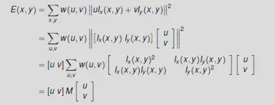
For small displacements $(u,v)$
$E(x,y)=[u\ v]M[u\ v]^T$
$M$: symmetric, positive definite $\Rightarrow$ eigenvalue decomposition possible.
Structure of the second-moment matrix
$M=\begin{pmatrix}A,C;C,B\end{pmatrix}$
with:
$A=\left(\frac{\partial I}{\partial x}\right)^2 \otimes w ; B=\left(\frac{\partial I}{\partial y}\right)^2 \otimes w ; C=\left(\frac{\partial I}{\partial x}\frac{\partial I}{\partial y}\right)\otimes w$
$w$: Gaussian window (isotropic).
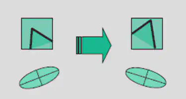
A corner is characterized by a large variation of $E$ in all directions of $(x,y)$.
$\Rightarrow$ Compute the eigenvalues of $M$.
Corner response
Instead of computing the eigenvalues, we can compute:
$\det(M)=AB-C^2=\lambda_1\lambda_2$
$\text{trace}(M)=A+B=\lambda_1+\lambda_2$
and define the response:
$R=\det(M)-k,\text{trace}(M)^2$
Values of $R$:
- positive near corners,
- negative near edges,
- small in flat regions ($k=0.04$).
$\Rightarrow$ corners / interest points = local maxima of $R$.
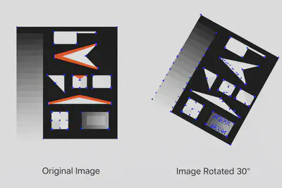
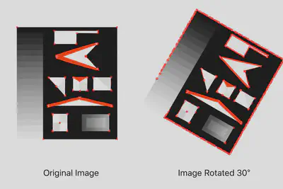
Invariant by rotation: even after rotation, the matrix shape is unchanged, so the eigenvalues and the response $R$ are unchanged.
Not invariant by scale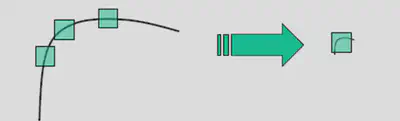
Potential solution: compute Harris response at multiple scales (Harris–Laplace).
PART F — From Features to Tracking
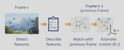
Feature-Based Tracking Pipeline
Frame t:
- Detect features
- Describe features
- Match with previous frame
- Estimate motion (R, t)
Repeat continuously.
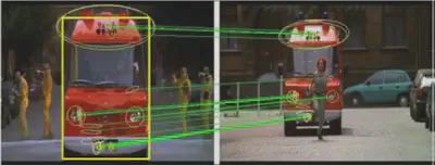
Feature Matching
Features are compared using descriptors.
Goal:
- Find correspondences between frames
This enables motion estimation.
Example: SIFT (Scale-Invariant Feature Transform)
SIFT provides:
- Scale invariance
- Rotation invariance
- Robust descriptors
Widely used in classical computer vision.
SIFT Pipeline
- Build Gaussian pyramid (multi-scale representation)
- Compute Difference of Gaussians (DoG)
- Detect keypoints
- Assign orientation
- Compute descriptor from local gradients
Build Gaussian pyramid, compute DoG and detect keypoints
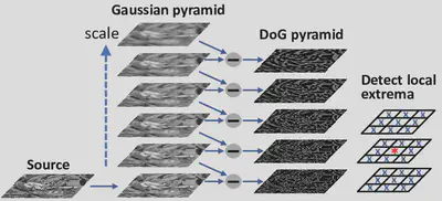
To obtain scale-independent descriptors, the image is resampled multiple times (building a “pyramid”).
The Gaussian difference is more efficient than a Laplacian calculation for each level.
Assign orientation and compute descriptor
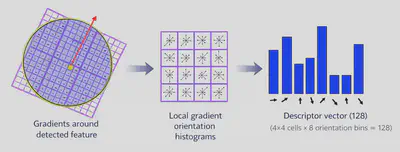
The descriptor is a histogram of local gradients around the keypoint, weighted by a Gaussian window.
PART G — From 2D Features to 6DoF Tracking
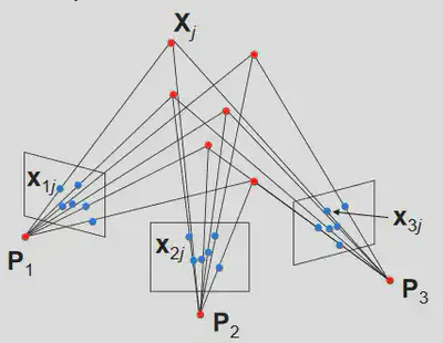
The PnP Problem (Perspective-n-Point)
If we know:
- 3D world points
- Their 2D projections in the image
We can solve for camera pose (R, t).
This is central to many AR systems.
Visual Odometry
If no 3D map is available:
- Track motion between consecutive frames
- Estimate relative movement of the camera
Used in SLAM systems.
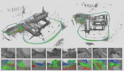
SLAM in XR
Modern headsets use SLAM:
- Simultaneous Localization and Mapping
- Build a map of the environment
- Track the headset within that map
Examples:
- ARKit
- ARCore
- Meta Quest inside-out tracking
PART H — Tracking in Modern XR Systems
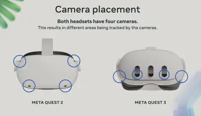
Inside-Out Tracking (Meta Quest)
Uses multiple cameras + IMU to:
- Track headset position
- Track controllers
- Map environment
Fully vision-based.
Optical Tracking (Vicon/OptiTrack)
Uses external cameras to track reflective markers.
Very accurate but requires a dedicated setup.
Hybrid Tracking Systems
Combine:
- Vision
- IMU
- Depth sensors
To improve robustness and reduce drift.